Traffic density estimation from probe vehicles
ProbeDensity estimates road congestion using only smartphone GPS and accelerometer data collected from vehicles on the road. It turns probe trajectories into link-level traffic density predictions through a full simulation-to-serving pipeline.
The project covers simulation-based data generation, feature engineering, model comparison, real-time ingestion, spatial matching, multi-probe aggregation, storage, and live visualization.
Why is this hard?
Each probe vehicle captures only a partial view of the surrounding traffic state.
Traffic density — vehicles per kilometer — is the fundamental measure of road congestion. But measuring it traditionally requires loop detectors, cameras, or radar embedded in the road, which are expensive and cover only major corridors.
Probe vehicles (taxis, ride-hails, smartphones) are everywhere, but each probe only sees its own trajectory. A car driving at 50 km/h could be in light traffic or moderate traffic — the speed alone doesn't tell you. The FD (Fundamental Diagram) speed-density relationship is degenerate in the free-flow regime: many densities map to nearly the same speed.
This project asks: can car-following behavioral patterns — acceleration variance, braking frequency, speed oscillations — break through that degeneracy?
Car-following theory meets gradient boosting
Speed alone is ambiguous. Density shows up more clearly in interaction patterns.
Car-following models such as IDM and Newell suggest that a vehicle's acceleration depends on spacing and relative speed to the leader. As density rises, those interactions become more frequent and leave visible traces in the trajectory: more braking events, higher acceleration variance, stronger speed oscillations, and longer stop behavior.
The system converts those signals into 31 handcrafted trajectory features spanning speed statistics, acceleration patterns, braking, stops, lateral dynamics, FFT, and sample entropy, then trains XGBoost to map them to density. In the deployed single-probe runtime path, the model also receives num_lanes and speed_limit, giving a 33-input inference vector (31 handcrafted + 2 road conditions). For the multi-probe case, the method then works in two stages: an aligned aggregated-feature XGBoost for the research setting, and a link-level Bayesian fusion system that keeps the pipeline usable when real probes arrive with mismatched traversal boundaries.
Link-based 1 km
Chain consecutive road links until 1 km, then extract features and predict.
Aligned Multi-Probe Study
Research setting where multiple probes observe the same 1 km slice and can be fused directly.
Link-Level Fusion Layer
Deployment-safe aggregation for probes with different traversal boundaries.
MAE 1.78 aligned vs 2.18 deployed
Deployable link-level fusion stays close to the aligned research setting while handling unequal traversal windows (R² 0.964 vs 0.951).
Smartphone to density map, end to end
The system has two halves: an offline ML pipeline that trains on SUMO simulation data, and an online serving pipeline that processes live smartphone telemetry into link-level density estimates.
graph TB
    subgraph Offline["Offline ML Pipeline"]
        A[SUMO Scenario Gen] --> B[FCD Trajectory Collection]
        B --> C[Edie Ground Truth]
        C --> D[31-Feature Engineering]
        D --> E[Model Training & Comparison]
        E --> F[Multi-Probe Study]
    end

    subgraph Phone["Smartphone"]
        G[GPS + Accel 1Hz] --> H[30s Local Buffer]
        H --> I["POST /ingest (bulk)"]
    end

    subgraph Server["Backend Server"]
        I --> J[Kalman Fusion]
        J --> K[GIS Link Match]
        K --> L["LinkBuffer (1km)"]
        L --> M[Trajectory Features + Road Conditions]
        M --> N[XGBoost]
        N --> O[Bayesian CF Ensemble]
    end

    subgraph Out["Output"]
        O --> P[(PostgreSQL)]
        O --> Q[Leaflet Map]
        O --> R[Kafka / Pub-Sub]
    end

    E -.->|trained model| N
    F -.->|fusion logic| O
    K -.->|auto lanes, speed_limit| L
What happens when a phone sends data
sequenceDiagram
    participant Phone as Smartphone
    participant Server as Backend
    participant GIS as LinkMatcher
    participant LB as LinkBuffer
    participant ML as XGBoost
    participant Ens as Ensemble
    participant Map as Map / DB

    Phone->>Phone: Collect GPS+Accel (1Hz)
    Phone->>Phone: Buffer 30 samples
    Phone->>Server: POST /ingest (bulk)

    loop Each sample
        Server->>Server: Kalman fusion (server-side)
        Server->>GIS: match(lat, lon)
        GIS-->>Server: link_id, lanes, speed_limit
        Server->>LB: Accumulate FCD + distance
    end

    alt Distance >= 1km
        LB-->>Server: LinkTraversal
        Server->>ML: trajectory features + road conditions → density
        ML-->>Server: density, cf_score
        Server->>Ens: Register per link
        Ens-->>Server: Bayesian link aggregation
        Server->>Map: Store + push
        Server-->>Phone: Prediction
    else Accumulating
        Server-->>Phone: Status
    end
A GUI to run experiments, compare models, and inspect failures
The offline pipeline is organized around a dashboard so experiment work becomes practical: generate scenarios, tune feature groups, choose model families, resume from saved assets, and inspect evaluation output without manually rewriting configs for every run.
The research needed an operating surface built for repeated experiments.
The project has many interacting knobs: scenario count, probes per scenario, feature subsets, FD residual options, model families, and evaluation targets. The dashboard turns those into a repeatable experiment surface with a repeatable workflow.
It also makes analysis faster after training. Each run keeps its own history, evaluation card, scatter plot, and feature-importance view, so model behavior stays visible throughout the workflow.
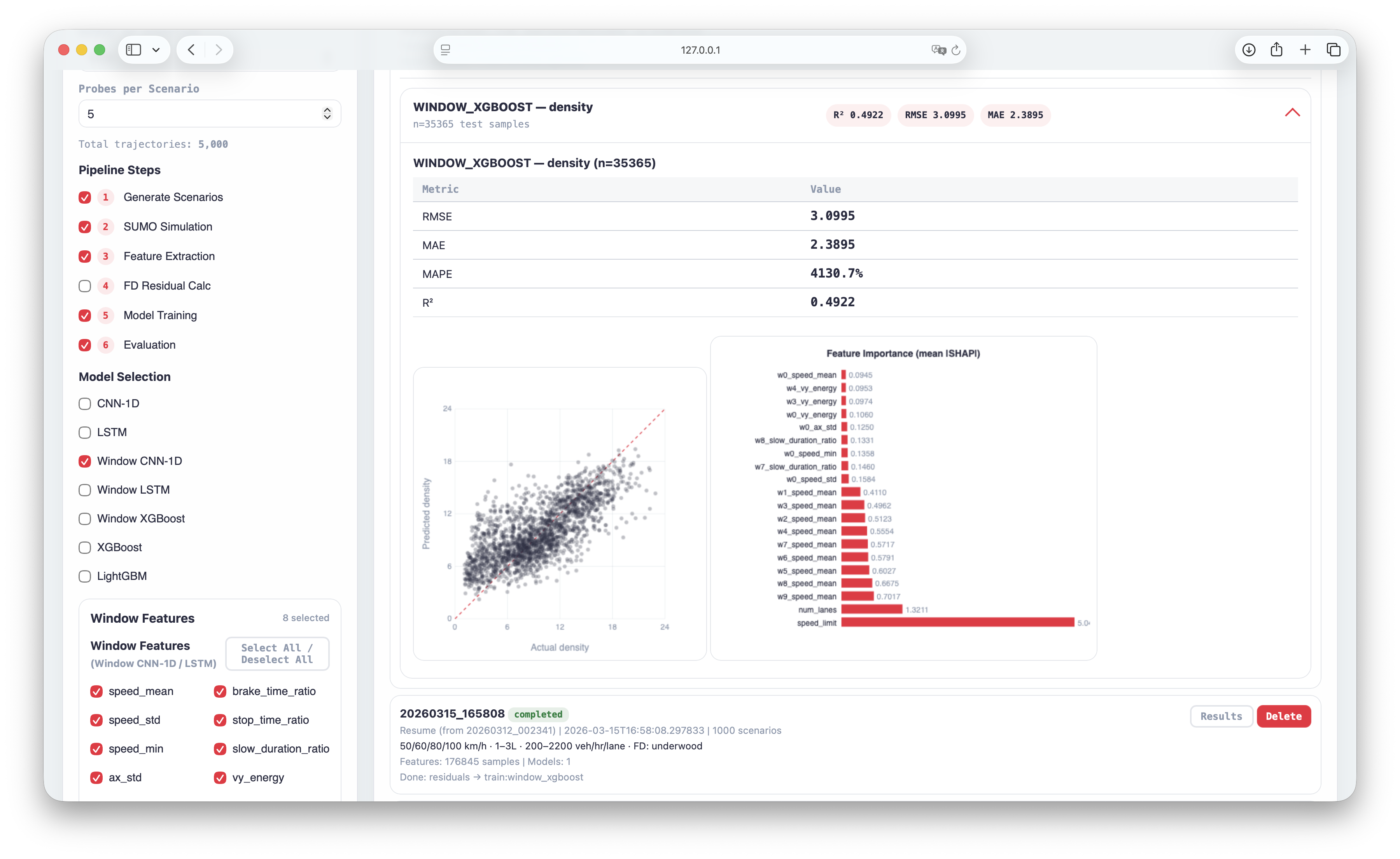
Scenario controls stay on the left, while completed runs reopen with inline metrics, scatter plots, and feature importance.
Open pipelineHosted server is view-only. Local runs unlock training and execution.
Scenario setup and resumable runs
Generate from scratch, resume from scenarios, FCD, features, or saved models, and tune demand, lanes, speed limits, and vehicle distributions without hand-editing configs.
Inline evaluation and model diagnostics
Open run history, compare per-model metrics, read actual-vs-predicted scatter plots, and inspect feature importance from the same dashboard after training.
Aligned fusion goes higher, deployable fusion stays usable
The project now reports two different result lines. The aligned research setting assumes multiple probes describe the same 1 km slice, while the deployable road-network setting must fuse unequal traversals only after per-probe prediction.
| Probes | MAE | MAPE | R² |
|---|---|---|---|
| 1 probe | 2.50 | 39.7% | 0.934 |
| 2 probes | 2.16 | 32.5% | 0.947 |
| 3 probes | 2.00 | 28.7% | 0.954 |
| 5 probes | 1.78 | 24.6% | 0.964 |
MAE = 1.78 veh/km/lane means about 2 vehicles per km per lane error across a density range up to ~67 veh/km/lane. This is the ideal same-slice setting where all probes describe the same 1 km target through an aggregated-feature XGBoost formulation.
| Method | N=1 | N=2 | N=3 | N=5 |
|---|---|---|---|---|
| Simple mean | 2.46 (0.935) | 2.30 (0.946) | 2.23 (0.949) | 2.18 (0.952) |
| CF-softmax | 2.46 (0.935) | 2.28 (0.947) | 2.21 (0.950) | 2.15 (0.953) |
| Bayesian+CF | 2.59 (0.928) | 2.36 (0.943) | 2.27 (0.947) | 2.18 (0.951) |
CF-softmax and Bayesian+CF land within ~0.03 MAE of each other at N=5, and both converge on R² ≈ 0.95. Bayesian+CF is the deployed fusion rule because it exposes the per-link posterior uncertainty the map display and downstream aggregation need.
MAE 2.50 to 1.78 from 1 to 5 probes
The aligned same-slice setting shows the value of multi-probe observation: MAE drops by 29% and MAPE by 15 points as probe count increases.
Bayesian+CF reaches MAE 2.18 at 5 probes
Different vehicles cover different cut points, so the system predicts each traversal first and then fuses them on the overlapping links they share (R² 0.951).
N=5 fusion methods stay close
Simple mean, CF-softmax, and Bayesian+CF land within ~0.03 MAE of each other once multiple unequal traversals are available; Bayesian+CF is chosen in deployment for its per-link uncertainty output.
How each subsystem actually works
Data Pipeline & ML Dataset209K samples · 31 handcrafted features · GroupKFold
From simulation to training set: 49K SUMO scenarios become 209K probe trajectories, then flow through feature extraction and leakage-safe validation.
49,000 SUMO scenarios generate 209K floating-car trajectories (6 channels × 1Hz). Each scenario parameterizes demand (200–6000 veh/h), speed limit (30–100 km/h), and lane count (1–3). Ground truth density is computed via Edie's generalized definition over the full time-space region.
Feature extraction runs through a registry pattern — each of 31 handcrafted trajectory features is a decorated function selected by YAML config. This lets experiments toggle features without code changes. In the deployed runtime path, num_lanes and speed_limit are added on top of those trajectory features. Training uses GroupKFold by scenario_id to prevent data leakage between probes from the same road.
All stages write to versioned run directories with manifest tracking. The ML pipeline dashboard supports resuming from any stage — retrain on existing features, re-evaluate a saved model, or filter by road conditions.
| Samples | 176,845 |
|---|---|
| Scenarios | 35,000 × 5 probes |
| Channels | VX, VY, AX, AY, speed, brake |
| Features | 31 handcrafted + 2 road inputs = 33 total |
| Validation | GroupKFold by scenario_id |
| Storage format | Parquet (tabular) + NPZ (timeseries) |
Real-Time Streaming & IngestionKalman → GIS → LinkBuffer → Fan-out
Serving path: buffered phone telemetry is fused, matched, accumulated, scored, then fanned out without making any one downstream dependency a blocker.
The smartphone buffers 30 seconds of GPS+accelerometer at 1Hz locally, then sends a bulk POST to reduce network calls by 30×. The server processes each sample through:
| GIS matching | Grid index (0.001° cells) reduces O(2.2K) → O(9 cells) |
|---|---|
| Re-match skip | 30m threshold eliminates ~90% of GIS calls |
| Bulk ingest | 30s batch reduces HTTP calls 30× vs per-sample |
| Sticky link | Prevents GPS jitter from triggering false traversals |
| Graceful degradation | DB/Kafka/GIS each optional — prediction always available |
Database Schema & Rolling Link Aggregationasync SQLAlchemy · 5 ORM models · 15-min link window
Storage model: per-probe predictions stay preserved, while each road link keeps a rolling aggregation record that opens, updates, freezes, and expires.
Async SQLAlchemy + asyncpg with 5 ORM models. EnsembleResult tracks multi-probe aggregation per link with a 15-minute rolling window (HCM analysis period).
flowchart LR
    RL[RoadLink\nlink_id · road_rank\nlink_length_m · lanes] -->|has| ER[EnsembleResult\nensemble_density\nprobe_count · is_frozen]
    RL -->|has| PR[Prediction\ndensity · cf_weight\ntraversal_time]
    ER -->|aggregates| PR
    PR -->|contains| FCD[FCDRecordRow\ntime · speed · brake]
Ensemble lifecycle: New probe prediction → find active ensemble for that link (or create) → compute Bayesian link density → update window_end. If no new probe within 15 min → freeze. Frozen ensembles are garbage-collected after 1 hour.
Stage 1 · Aligned Multi-Probe Aggregationsame-slice research setting · MAE 1.78 / MAPE 24.6% (R² 0.964)
Research layer: when probes observe the same slice, their handcrafted features are aggregated into one fixed-length vector before XGBoost prediction.
The aligned model aggregates each selected probe's handcrafted feature values into a single tabular input. The model receives the mean and standard deviation of each feature across probes.
Example: if three probes have speed_mean = 42, 48, 45, the aligned input stores speed_mean_mean = 45 and speed_mean_std ≈ 2.45. If their traversal times are 62, 71, 68 seconds, the aligned input stores traversal_time_mean = 67 and traversal_time_std ≈ 3.74.
This makes the aligned model a tabular aggregated-feature XGBoost. Its strength appears once multiple probes are present, because the standard-deviation terms begin to describe how differently the probes experience the same 1 km slice. This formulation reaches MAE 1.78, MAPE 24.6% (R² 0.964) at 5 probes.
Stage 2 · Overlap-Aware Link Fusion for Mismatched Traversalsdeployed 5-probe system · MAE 2.18 / MAPE 37.2% (R² 0.951)
Deployment layer: once probes stop sharing identical 1 km observation windows, the system predicts each traversal first, then aggregates those densities through the road links their windows overlap.
In deployment, vehicles do not stop and start their traversal window at the same place. Their measurements are misaligned but still partially overlapping, so requiring identical segments would throw away most usable multi-probe evidence.
The system registers each traversal's density on the road links it covers, keeps a 15-minute rolling ensemble per link, and recomputes the aggregate with a Bayesian posterior whose observation noise shrinks as CF intensity rises. In practice, traversals that show stronger car-following behavior are treated as lower-noise observations inside the shared link window.
t, then aggregate only the traversals whose windows overlap the same link.CI/CD & Cloud DeploymentGitHub Actions → Cloud Run · 0–2 auto-scaling
Release path: every push is checked, every release is containerized, and production automatically scales down when idle.
CI runs on every push (lint → type check → pytest matrix → Docker build smoke test). CD triggers on GitHub Release: build & push to Artifact Registry → deploy to Cloud Run (0–2 auto-scaling) → verify health. Code releases and model/GIS asset bundles are versioned separately.
What Worked, What Didn't, and What Comes Next
The strongest parts are the experiment workbench, the deployable density-estimation system, and the road-network aggregation logic that keeps the method usable outside the aligned research setting. The remaining gaps are concentrated in simulation fidelity and sensor assumptions.
In the aligned 5-probe, 1 km experiment, aligned multi-probe aggregation reaches MAE 1.78, MAPE 24.6% (R² 0.964). The second contribution is the deployable version: an overlap-aware Bayesian link-fusion system that still delivers MAE 2.18, MAPE 37.2% (R² 0.951) in the deployed 5-probe setting once probes stop sharing the same traversal boundaries.
Trained on 49K SUMO scenarios spanning density 0–67 veh/km/lane. XGBoost on 33 inputs (31 handcrafted + num_lanes + speed_limit) is the runtime model. Multi-probe aggregation cuts MAE another 29% on top.
Right now the system is presented in a browser-first form, so the phone behaves mostly like a thin client. If this moves into an installed mobile app or an in-vehicle system, more of the buffering, sensor fusion, feature preparation, and filtering can run locally before upload. That would reduce server load, network cost, and end-to-end latency without changing the core model idea.
Links are short and variable, so a fixed time window does not map cleanly onto a stable road segment. The system therefore chains consecutive links until a traversal reaches about 1 km, then predicts at that road-linked unit. Unequal traversal boundaries are a direct consequence of deployable link measurement.
The current phone-only system infers spacing indirectly from motion features. Direct headway or forward-gap signals from ADAS or connected vehicles would make that information observable instead of latent, making spacing-aware sensing the highest-upside next research direction.
Inspect the running pipeline
This block is for moving, not reading. Start from the live console, then jump into the surface that explains, tests, or inspects one part of the deployed system.
Runtime Console
Open the single best starting point for the live demo. It pulls the current snapshot, service health, map feed, and the runnable paths into one operational surface.
If you only click one thing on this page, this is the one that tells you whether the deployed system is actually alive.
Open live consoleLink Density Map
See deployed link-level ensemble density on the road network, color coded by traffic state with probe count and CF weight visible per link.
Data Ingestion Test
Send raw GPS and accelerometer payloads into POST /ingest and
watch the hosted pipeline go from Kalman fusion to GIS match, buffering, inference, and ensemble.
OpenAPI Reference
Inspect the real FastAPI schema for /ingest,
/predict, and /map/links/* endpoints, with request and response shapes
ready for live testing.